
What reaction time reveals about suprathreshold hearing
Listening Beyond the Audiogram
An audiogram answers an important but narrow question: how faint can a tone be before it disappears? It does not tell us how well a listener represents the spectral and temporal detail of a sound that is already audible. That distinction matters in daily life. Listeners with similar pure-tone thresholds do not necessarily find speech in noise equally easy.
Here I use reaction time (RT) to examine that second part of hearing. The task requires only a button press when an audible spectrotemporal ripple changes. The analysis is less simple: reciprocal RT provides a measure of promptness, separate transfer functions describe spectral and temporal performance, and a Bayesian ANOVA checks the result without imposing those curve shapes. The data compare listeners with normal hearing with three groups with genetic hearing loss: COL11A2, STRC, and TECTA.
1. A button press as a measure of hearing
Each trial begins with a static noise. At an unpredictable moment it changes into a dynamic spectrotemporal “ripple.” The listener’s task is to press a button as quickly as possible after detecting that change. Reaction time is measured from the onset of the ripple to the button press.
The ripple varies along two dimensions: temporal velocity (in Hz), which describes how quickly its pattern moves across frequency, and spectral density (in cycles/octave), which describes how closely its peaks are spaced. Most conditions combine a non-zero velocity with a non-zero density, so both dimensions vary. Only conditions on the axes isolate one dimension:
dens == 0, vel ≠ 0→ only temporal velocity changesvel == 0, dens ≠ 0→ only spectral density changesvel == 0, dens == 0→ catch condition: the sound remains static
Each condition is presented 5–10 times, providing repeated reaction-time measurements across the velocity × density grid.
Before analysis, I apply two rules:
| Rule | Value | Reason |
|---|---|---|
| Drop RT ≤ | 0.150 s | Too fast to reflect actual stimulus-driven detection — anticipatory guesses |
| Cap RT > | 3.0 s → 3.0 s | Treated as a non-detection; sets a floor on promptness rather than discarding the trial |
Slow trials are not discarded. They are left-censored on the promptness scale: the model records only that promptness was at or below 1/3 Hz. This preserves the non-detection without pretending to know its exact RT and is used explicitly in the Bayesian ANOVA below.
Every remaining RT is then transformed:
promptness = 1 / RT (units: Hz)
The LATER model provides the rationale for using reciprocal rather than raw RT.
2. Why reciprocal RT: the LATER model
LATER — Linear Approach to Threshold with Ergodic Rate — is a simple race-to-threshold account of decision time originally proposed by Carpenter and Williams for saccadic eye movements (Carpenter & Williams, 1995, Nature 377:59–62), and since generalised to manual and vocal RT tasks across psychophysics.
The model says: on every trial, an internal decision signal rises linearly
from a starting level S0 to a fixed threshold ST. The rate of rise, r,
is not constant — it varies from trial to trial, drawn from a Gaussian
distribution. Reaction time is simply the time it takes the signal to cover
the distance from start to threshold at that trial’s rate:
RT = (ST − S0) / r
Because RT is inversely related to the rate, 1/RT (promptness) is approximately Gaussian under this model; raw RT usually has a long right tail. On a reciprobit plot (probit probability against 1/RT), LATER predicts a straight line. A change in the rate variance rotates that line (a swivel), whereas a change in its mean translates it (a shift).
This choice has three practical consequences:
- It justifies using promptness instead of RT as the dependent variable used in the models below. Promptness is generally closer to a symmetric distribution than raw RT, without requiring an unrelated transformation.
- It gives the RT-capping rule a mechanistic interpretation. A trial where the listener never reaches threshold within 3 s isn’t an arbitrary cutoff. Censoring rather than deleting preserves the information that a response did not occur within the analysis window.
- It frames “faster median RT” as “more efficient evidence accumulation”, while avoiding a direct interpretation of the skewed RT scale. It is still a behavioural measure, however: attention, motor speed, and decision strategy can also affect it.
LATER therefore motivates promptness as the response variable. It does not, by itself, make reaction time a pure measure of auditory processing; that interpretation depends on the task design and comparisons between conditions.
3. From individual responses to a transfer function
A single response says little. The useful object is promptness as a function of stimulus strength, estimated separately for temporal velocity and spectral density. Together these curves form the modulation transfer function (MTF).
The model is a hierarchical Bayesian model fit per group in Stan
(stm_model.stan), with two transfer functions sharing a common likelihood:
y_i ~ Student-t(ν, μ_i, σ)
A Student-t likelihood limits the influence of occasional outlying responses.
Temporal MTF — a Gompertz CDF in log-velocity space, rising from near-zero promptness at low velocities to an asymptote α at high velocities:
μ_i = α_s · exp( −exp( k_t · (log|vel_i| − θ_s^t) + c ) )
Spectral MTF — a logistic function in log-density space, falling from a high plateau at low densities toward zero as the ripple becomes too dense to resolve:
μ_i = α_s · ( 1 − 1 / (1 + exp(−(2 log 9 / ω_s^s) · (log(dens_i) − θ_s^s))) )
Both curves use three subject-level parameters, partially pooled within each group. That pooling is especially useful here because the groups contain only 4–8 listeners:
| Symbol | Name | Units | Meaning |
|---|---|---|---|
| α | alpha | Hz | Asymptotic maximum promptness — the plateau |
| θ | theta | log(Hz) or log(cyc/oct) | Threshold: stimulus level at half-maximum promptness |
| ω | omega | log-units | Transition width — how gradual the slope is |
Because θ lives in log-space (matching the log-encoded stimulus axes), it’s exponentiated back into physical units for reporting:
exp(ttheta) = temporal fidelity   (Hz)       — velocity at half-maximum promptness
exp(stheta) = spectral edge       (cyc/oct)  — density at half-maximum promptness
A subject-level snippet of the Stan likelihood block makes the two-branch structure explicit:
if (is_temporal[i] == 1) {
    real exponent = (log_neg_log_09 - log_neg_log_01) / tomega[s[i]]
                    * (v[i] - ttheta[s[i]]) + log_neg_log_05;
    mu = alpha[s[i]] * exp(-exp(exponent));
} else {
    real logit_arg = -two_log_9 / somega[s[i]] * (d[i] - stheta[s[i]]);
    mu = alpha[s[i]] * (1 - 1.0 / (1 + exp(logit_arg)));
}
y[i] ~ student_t(nu, mu, sigma);
Four chains, 1000 warmup + 1000 sampling iterations, adapt_delta = 0.99
(CmdStanPy compiles and fits this in roughly 10–40 minutes for four groups).
A good fit shows zero divergent transitions, R-hat ≈ 1.00, and effective
sample size > 400 per parameter — the same checklist you’d use for any HMC
model, nothing exotic here.
The resulting group curves look like this:
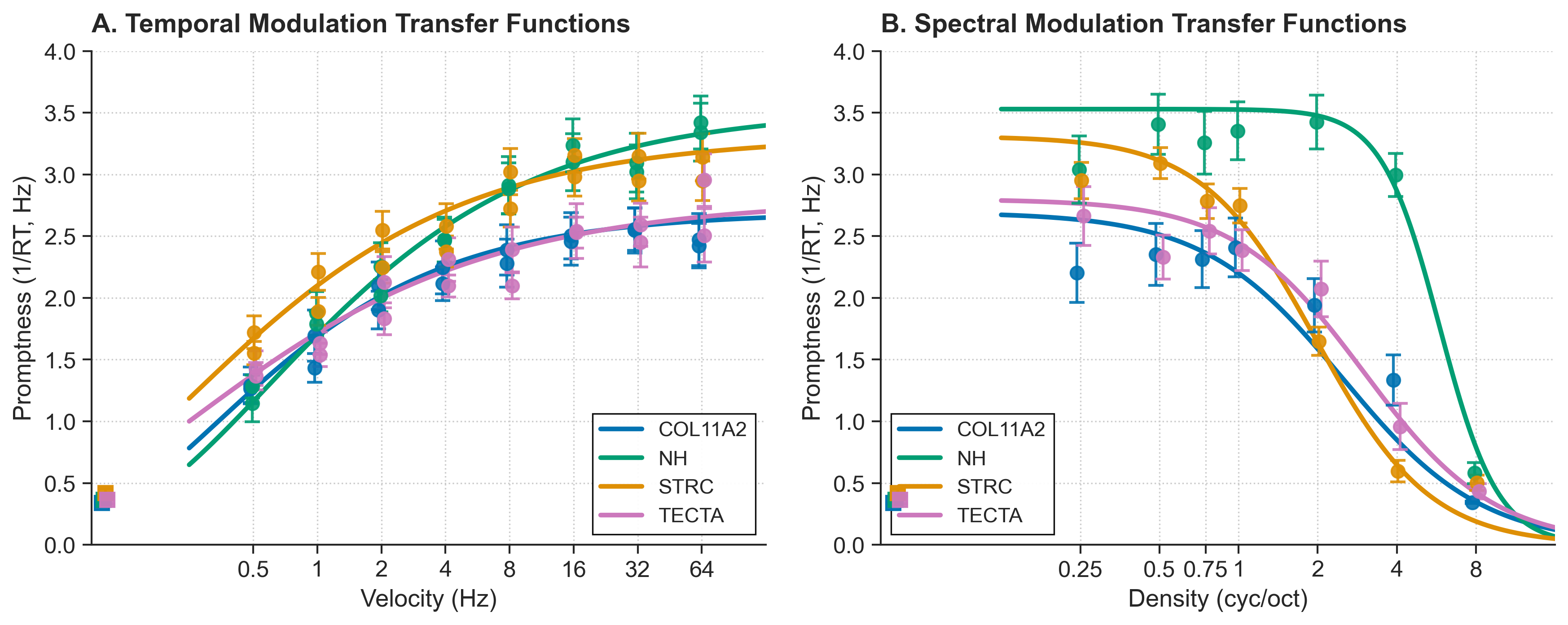
In the temporal panel, a higher θ shifts the rising curve to the right: a higher velocity is needed to reach half-maximum promptness. In the spectral panel, a higher θ shifts the falling edge to the right and indicates that denser ripples remain resolvable. In either panel, α sets the response plateau and ω determines how gradual the transition is.
4. Spectral and temporal performance can diverge
A single score would be simpler, but it would hide differences between spectral and temporal performance. Those differences may help distinguish the effects of different cochlear pathologies.
In this dataset, despite all three hearing-loss groups carrying a genetic diagnosis and broadly comparable audiograms, the MTF profiles tell different stories:
- STRC (DFNB16) shows a predominantly spectral deficit — consistent with dysfunction of the cochlear amplifier (outer hair cell / stereocilin pathology), which primarily degrades frequency selectivity rather than timing.
- TECTA (DFNA8/12) and COL11A2 (DFNA13) show similar combined spectral and temporal impairments, with COL11A2 showing the largest deficits overall.
Keeping temporal and spectral trials in separate transfer functions
(ttheta/tomega and stheta/somega) makes that distinction visible.
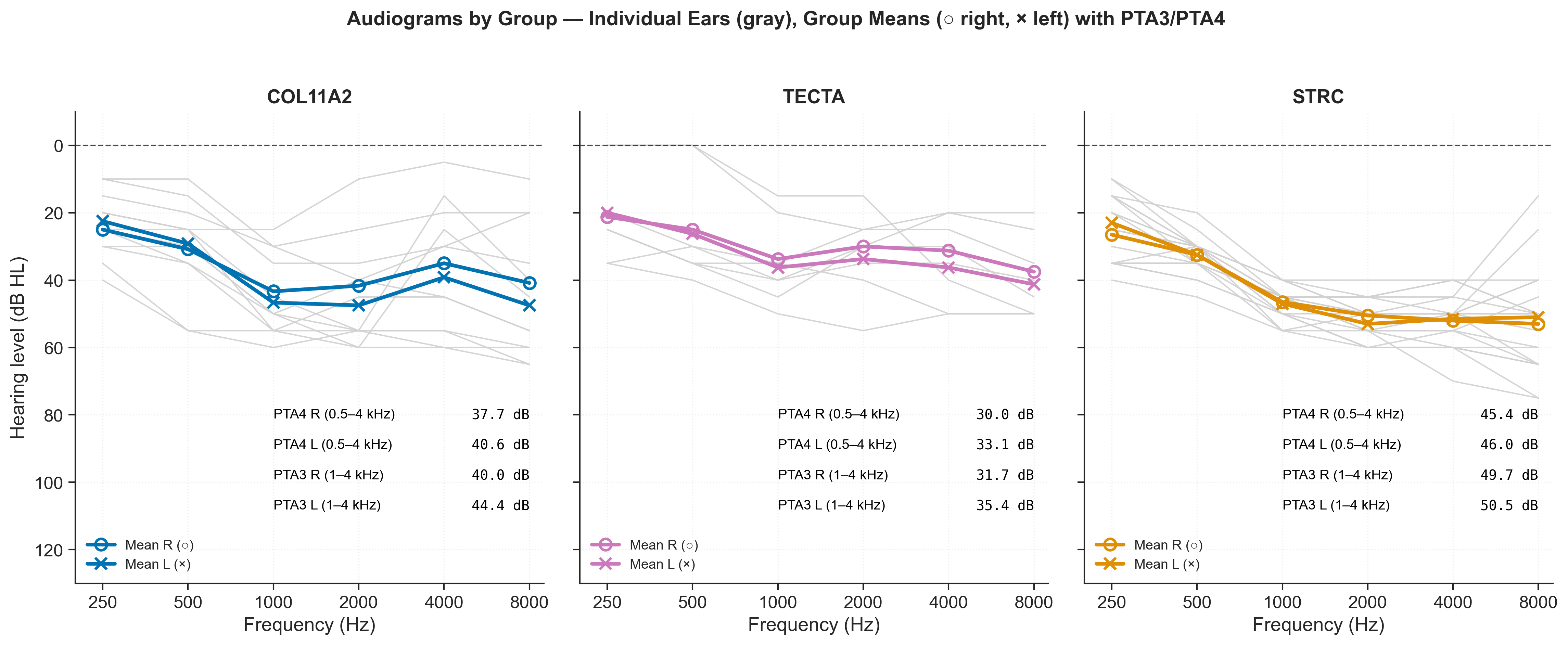
The audiograms for the same three groups, for comparison — note how similar they look despite the MTF differences above:
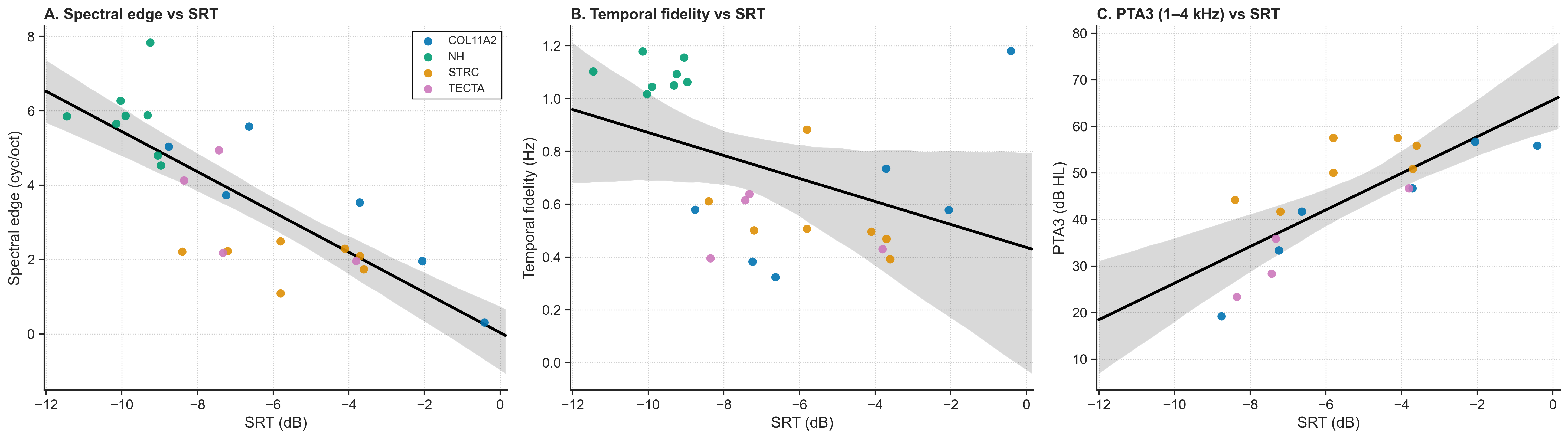
I then use a series of OLS regressions (with HC3 robust SEs) to test whether
spectral_edge (exp(stheta)) and
temporal_fidelity (exp(ttheta)) predict speech-reception threshold
(SRT) in noise — measured independently with the Dutch Matrix
speech-in-noise test — over and above audiometric hearing level (PTA) and
age:
SRT ~ PTA3_z + Spec_z + Temp_z + Age_c + C(group)
In these data, spectral resolution is more strongly related to SRT than
temporal resolution. Much of that association is shared with audibility
(PTA), as the residualised model shows after removing the effects of PTA and
age from Spec_z and Temp_z:
These measures add information that is absent from a pure-tone audiogram and do not require speech material. Whether they can guide individual rehabilitation is a separate question that will require prospective evidence.
5. Checking the curve model with a 3-way Bayesian ANOVA
The Gompertz and logistic functions impose particular curve shapes. As a check, I also ask whether promptness differs across velocity × density conditions when every condition has its own cell mean. This 3-way Bayesian ANOVA (velocity × density × subject) follows the approach in Veugen et al. (2022, DOI: 10.1177/23312165221127589), itself built on the censored-ANOVA framework in Kruschke’s Doing Bayesian Data Analysis (2nd ed., Ch. 20).
The original: JAGS
The reference implementation is a MATLAB + JAGS model
(jags_anova3xway_censor.m / RunModel.m) — Gibbs sampling, sum-to-zero
deviation-coded effects (b0, b1, b2, b3, b1b2, b1b3, b2b3, b1b2b3), and
explicit left-censoring of non-responses via an isCensored indicator vector
fed straight into the JAGS data block. The original run used the
fixed-σ, Student-t branch of the model (varSigma = false) — a single
shared noise SD per group, with the t-distribution’s ν parameter providing
robustness to outliers.
The port: Stan
The Stan port (model_rt_3way_cellsd_s2z.stan) changes one important model
choice. The JAGS analysis used a shared σ, which avoids updating a separate
scale parameter for every velocity × density × subject cell. With HMC, the
cell-specific version is practical, so the Stan model uses cell-specific
σ with a Normal likelihood (the equivalent of varSigma = true).
There are three reasons for not retaining the Student-t likelihood:
- The outlier-prone trials it was designed to absorb (anticipatory guesses, non-responses) are already handled upstream by the 150 ms floor and the 3 s left-censoring — so there’s little heavy-tailed residual left for ν to model.
- With only 5–15 trials per (velocity, density, subject) cell, ν is barely identifiable from the data anyway — the model collapses toward Normal in practice regardless.
- The heteroscedasticity across cells (tight, fast responses near ceiling; noisy, slow responses near threshold) is a genuine feature of the data, not noise to be averaged away — and a single shared σ would force the model to under-fit both regimes simultaneously.
The other deliberate departure is the intercept prior. JAGS’s effectively
flat τ ~ Gamma(0.001, 0.001) is harmless for Gibbs sampling but creates
pathological geometry for HMC (Stan can wander into physically impossible
regions — negative promptness — and report divergences). The Stan version
uses a0 ~ Normal(y_mean, 5 · y_sd): still weakly informative — five SDs
either side of the observed grand mean covers essentially any plausible
value — but it keeps the sampler out of the tails where the geometry breaks
down. The two priors produce indistinguishable posteriors; only the sampler’s
behaviour differs.
The sum-to-zero centering itself is implemented as a Stan functions block
(center_sum_to_zero, center_sum_to_zero_2d, center_sum_to_zero_3d) that
takes raw, unconstrained effect parameters and re-centers them so that every
main effect and interaction sums to zero across its levels — the same
identifiability trick as deviation coding in classical ANOVA, just written
out explicitly because Stan has no built-in factor syntax:
vector center_sum_to_zero(vector x) {
    return x - mean(x);
}
The linear predictor itself reads exactly like the ANOVA decomposition it represents:
μ_i = a0 + a1[v] + a2[d] + a3[s] + a1a2[v,d] + a1a3[v,s] + a2a3[d,s] + a1a2a3[v,d,s]
with promptness_i ~ Normal(μ_i, σ_{v,d,s}) for observed trials and
left-censoring at 1/3 Hz for the capped ones — fit with 3 chains, 10,000
warmup, 6,667 sampling iterations per group.
The result is a less constrained check on the MTF result: group-level
heatmaps of promptness across the full velocity × density grid (using only
the fixed effects a0 + a1[v] + a2[d] + a1a2[v,d], deliberately excluding
subject terms to show the population-level pattern), plus marginal
spectrotemporal profiles with 95% highest-density intervals:
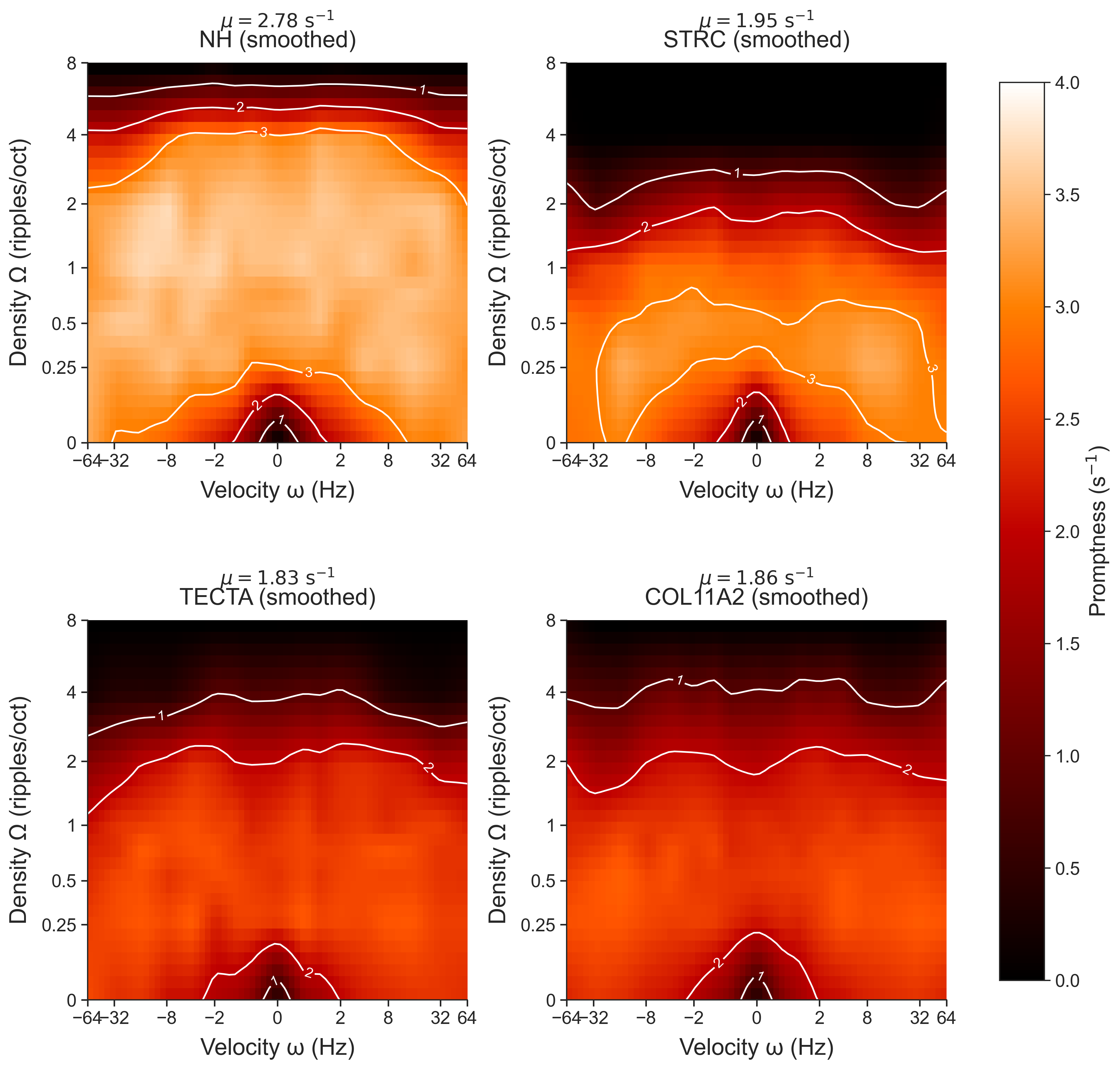
Here the smooth MTF and the cell-based ANOVA agree. That makes it less likely that the main group pattern is an artefact of the Gompertz or logistic curve shape.
6. Putting it together
The full pipeline has three branches that share one RT dataset and converge on one regression:
RT data (19,561 trials)
   │
   ├── Branch A — hierarchical MTF (Stan)         → α, θ, ω per subject
   ├── Branch B — 3-way Bayesian ANOVA (JAGS→Stan) → model-free confirmation
   │
   └── Branch C — Matrix speech-in-noise test      → SRT per subject
                                                          │
        spectral_edge, temporal_fidelity  ───────────────┘
                              │
                              ▼
                  SRT ~ PTA + Spec_z + Temp_z + Age + group
For a comparable analysis: collect RTs to clearly audible stimuli that vary along one dimension at a time; define the anticipatory and censoring limits before fitting the model; transform RT to promptness; fit separate transfer functions for each stimulus dimension; compare their predictions with a cell-based model; and only then relate the curve parameters to an independent outcome.
References
- Carpenter, R.H.S., & Williams, M.L.L. (1995). Neural computation of log likelihood in control of saccadic eye movements. Nature, 377, 59–62.
- Kruschke, J.K. (2015). Doing Bayesian Data Analysis (2nd ed.), Ch. 20: Metric Predicted Variable with Multiple Nominal Predictors. Academic Press.
- Veugen, L.C.E., et al. (2022). DOI: 10.1177/23312165221127589
- Stan Development Team. CmdStanPy documentation.